Click or tap a + to explore.
History of AI
Explore
For a complete history of AI see: Wikipedia.
The History of AI according to me:
The Day the World Changed (2022)
November 30, 2022 · ChatGPT arrives

On Wednesday November 30th, 2022, ChatGPT was announced, and the world has not been the same since.
Before ChatGPT, for most of us, AI was a term of Science Fiction or something that could play a good game of Chess.
And then ChatGPT came along and suddenly, anyone – anywhere – could talk with it (in text), ask questions, get useful answers, and it understood you and could follow your chain of thought.
It also knew a lot about every topic under the sun! It could write, create stories, tell jokes, write in the voice of a favorite author, write in different languages, translate, and even write computer code!
And with that, the revolution began.
A revolution, but one word at a time!†
When one asks ChatGPT a question, the answer appears gradually as if someone were typing it. But that isn’t just a display trick.
Ask ChatGPT:
What is a typo?And it does not come up with the answer and then display it.
Instead, its task is far more limited, it asks itself:
What is the most likely next word?
It displays the chosen word as the beginning of an answer.
What is a typo?
A
It has not found a full answer; it has only found the first word of an answer.
It then repeats the process, over and over, each time asking: What is the most likely next word?
What is a typo?
A typo
And then again:
What is a typo?
A typo is
and again:
What is a typo?
A typo is a
and again:
What is a typo?
A typo is a mistake
This continues until the most likely next word isn’t a word at all, but is an indication that the answer is complete. Then it stops.
What is a typo?
A typo is a mistake made while typing text, usually caused by a slip of the fingers on a keyboard or screen.
That this approach produces great results is a surprise to everyone involved.
To add variety, it actually doesn’t always pick the most likely next word, but randomly selects one of the most likely next words. You can ask the same question twice, exactly the same way, and you will likely get slightly different results each time. This is why.
This isn’t just how ChatGPT works. Other well-known Large Language Models (LLMs), including Claude from Anthropic, Gemini from Google, Llama from Meta, and DeepSeek, use this same basic approach.
Context Window and Memory
The question and its growing answer make up the context window. When the answer stops being generated, and one asks a new question, say "Give me some examples.", the original typo question, its answer, and the new question are all taken in with the goal of once again finding the next likely word, and then the next, and the next, until the next stop.
Through this ever growing context window, the AI understands new questions in the context of the previous questions and answers. This creates a form of memory where each new word generated not only is in response to the words of the immediate question, but is informed by the words of the entire series of questions and answers that came before.
This ability to draw on the preceding words of the question, and the words of the earlier questions and answers, comes from the AI’s attention mechanism.
Remarkably, this too operates at the word level, influencing the understanding of the words of the question in the context of the other words in the question and in prior questions and answers.
Generative Pre-trained Transformer
GPT, from ChatGPT, stands for:
Generative means it produces text, building a response one word at a time; technically, one token at a time, where a token can be a word, part of a word, or punctuation.
Pre-trained means it first learns patterns from large amounts of text, before post-training adapts it for tasks such as answering questions and following instructions.
Transformer is the neural-network architecture it uses; its attention mechanism helps it relate different parts of the text, such as connecting a pronoun with the person to whom it refers, or connecting a follow-up question to an earlier topic.
ChatGPT is an application allowing one to interact with an AI model in a conversational style. The original version used the GPT-3.5 model which is an example of a Large Language Model (LLM). LLMs are trained on vast amounts of text so that they can process and generate language. Most other LLMs also share the generative, pre-trained, transformer architecture even if they do not use it in their names.
How much text was it trained on?
The original ChatGPT was based upon the GPT-3.5 model. In a night-before-the-launch decision, the name was changed from “Chat with GPT 3.5” to simply “ChatGPT”. The 3.5 model was based upon GPT 3.0 with additions for coding. OpenAI hasn’t disclosed GPT-3.5’s exact training data, but GPT-3 had been trained on:
Around 225 billion words of text (300 billion tokens):
- 60% from a crawl of billions of web pages
- 22% from WebText2, a high-quality dataset covering highly upvoted content from Reddit.
- 16% from Book1 & Book2, two long-form Internet book repositories
- 3% from Wikipedia
The increment to GPT-3.5 included an undisclosed amount of high-quality computer code from open sources such as GitHub which heavily improved the model’s logic, reasoning, and programming capabilities.
Learn more: OpenAI's launch announcement · GPT-3 training data (pages 8–9) · What are tokens?
Before ChatGPT: ELIZA (1966)
1966 · The illusion of understanding
Fifty six years before ChatGPT, there was ELIZA.
ELIZA illustrates how engaging text conversations can be and how easily the illusion of understanding can be produced.
ELIZA is your psychotherapist, try it out:
Talk with ELIZA
A recreation of the classic DOCTOR conversation. Your conversation stays in this browser tab.
How ELIZA works
By implementing a few basic rules, ELIZA creates a sometimes convincing illusion of an intelligent conversation between a psychotherapist and their patient. Here is all it is doing:
- Clean up the input: Normalize capitalization and expressions such as “I'm” into “I am.”
- Look for keywords: ELIZA looks for words such as “remember,” “dream,” or “sorry” to choose a set of response rules. Some keywords have higher priority than others.
- Match a sentence pattern: A rule might recognize “I am ___” and capture whatever follows.
- Build a reply from a template: Insert the captured words and change pronouns — “my” becomes “your,” for example.
- Keep the conversation going: If nothing useful matches, use a general prompt or bring back something saved from an earlier remark.
These rules:
Pattern:  I am [something]
Reply:    How long have you been [something]?

Pattern:  My [something]
Reply:    Your [something]?
          Change “me” to “you.”
Together, they can produce:
You:      I am tired.
ELIZA:    How long have you been tired?
You:      For weeks. My work keeps me awake.
ELIZA:    Your work keeps you awake?
The illusion of understanding can be quite strong despite the simplicity of ELIZA’s rules. Modern AI systems are vastly more capable, have they crossed over into actual understanding? They seem to have. One lesson of ELIZA, however, is that people see understanding and presence easily.
Browser implementation: elizabot.js by Norbert Landsteiner (2005), based on Weizenbaum's ELIZA and DOCTOR rules. This port includes some later additions. Read about restoring the original ELIZA.
The Birth of AI (1955)
1955–1956 · Giving a field its name
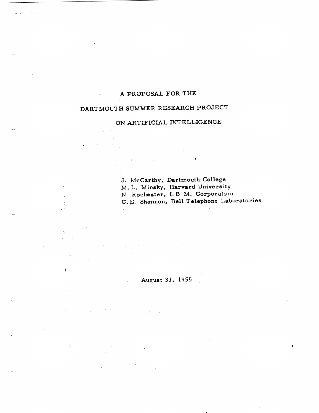
In 1955, a summer research project at Dartmouth College was proposed. The title was:
A PROPOSAL FOR THE
DARTMOUTH SUMMER RESEARCH PROJECT
ON ARTIFICIAL INTELLIGENCE
This is where the new field got its name. The meeting itself took place in the summer of 1956, in Hanover, New Hampshire.
The Logic Theorist
At the 1956 meeting, the Logic Theorist was introduced. In its early tests, it was able to prove 38 of 52 theorms drawn from the important book Principia Mathematica. This is an early example of Symbolic AI, which represents information using symbols and applies explicit rules to reason about them.
The new field of AI was off to a strong start.
Logic Theorist used heuristics — rules of thumb that guided its search toward promising proofs. Its successor, GPS (General Problem Solver), generalized this into means-ends analysis which is still important today.
Sources: McCarthy's account of Dartmouth · Newell, Shaw, and Simon's 1957 report · Stanford's history of AI.
Means–ends analysis
Means-ends analysis involves choosing actions that brings one closer to a goal (end), then setting subgoals (means) when needed.
Example:
- Goal: Print the document.
- Notice a problem: The printer is out of paper.
- Subgoal: Load paper into the printer.
- Complete the goal: Print the document.
In order to reach the goal, subgoals must be determined and resolved first.
Learn more: Newell, Shaw, and Simon's GPS report · Peter Norvig's GPS explanation · How Large Reasoning Models Solve Problems: A Mechanistic Study on Tower of Hanoi.
Computers and Programming (1950s)
To appreciate the initial advancements in Artificial Intelligence, it is worth remembering just how new, and few, computers were in the 1950s. The first commercial electronic computer was only just delivered in 1951. Across the entire decade, there were only a relative handful sold:
| Computer | Year | Total units sold |
|---|---|---|
| UNIVAC I | 1951 | 46 |
| IBM 701 | 1952 | 19 |
| IBM 650 | 1954 | ~2,000 |
| IBM 704 | 1955 | 123 |
In today’s dollars, the IBM 650, the inexpensive system on the list, would cost around $2.5 million and occupy as much space as a small industrial kitchen. The other systems were in the $10 million to $25 million range. And even the most advanced, the IBM 704, had processing power and memory capacity that a smart-card chip on a credit card in your wallet can match or exceed.
Programming Languages
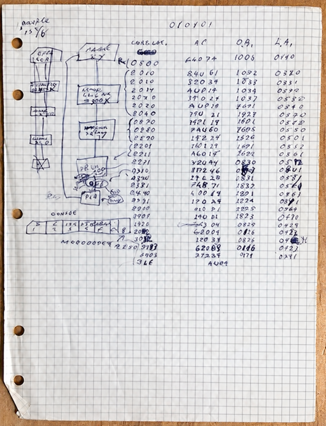
There were hardly any programming languages in the early 1950s. Most computers were programmed using their native machine languages or labeled versions of machine language called assembly language.
More about Machine and Assembly language (optional)
Modern computers (then and now) are stored-program systems. A series of instructions - a program - is stored in the computer's memory. The computer steps through those instructions, performing them one at a time.
Machine language. Instructions are encoded as numbers using binary digits - bits. This is machine language. A typical instruction contains a numeric operation code - an opcode - specifying what to do and an address specifying the memory location involved.
For example, for the IBM 704 computer, these instructions load a value, add another, and store the result:
| Opcode | Address | Explanation |
|---|---|---|
+0500 | 05000 | Load the value from location 5000 |
+0400 | 05001 | Add the value from location 5001 |
+0601 | 05002 | Store the result at location 5002 |
Assembly language. Programming in machine language can be tedious. Assembly language improves this by giving instructions readable names for operations and locations. Suppose we name those three locations for Balance, Payment, and New Balance. These same instructions might then be written:
| Operation | Location | Explanation |
|---|---|---|
CLA | BALANC | Load the balance |
ADD | PAYMNT | Add the payment |
STO | NEWBAL | Store the new balance |
CLA stands for “clear and add”: it clears the accumulator and adds the specified value, effectively loading it. ADD adds the second value, and STO stores the result.
A program called an assembler translates the Assembly Language to Machine Language for the machine to execute.
Sources: IBM 704 manual, pages 17–19, 73, and 91–92 · MIT's 1957 IBM 704 programming manual.
New programming languages arrived toward the end of the decade:
- Fortran (Formula Translation), released in 1957, made scientific and mathematical calculations easier to express.
- Cobol (Common Business-Oriented Language), designed in 1959, aimed at readable business programs that could run on different manufacturers' computers.
- Lisp (List Processing), developed by John McCarthy (from the Dartmouth Summer project) beginning in 1958, made symbolic expressions and lists central to programming.
Sources: IBM's Fortran history · Cobol manual and history · McCarthy's history of Lisp.
Neural Networks and the Perceptron
Just as we drew inspiration from birds for flight, we have drawn inspiration from the human brain for AI's neural networks (Artificial Neural Networks).
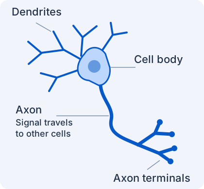
The biological neuron
The artificial neuron

An adult human brain contains some 86 billion neurons. Cortical neurons typically have around 10,000 incoming synaptic connections and a similar number of outgoing connections. Altogether, there are hundreds of trillions of synaptic connections in the brain.
From this biological inspiration, artificial neural networks (ANNs) have borrowed these ideas:
- Neurons receive and combine signals
- Connections are of various strengths
- Learning changes those strengths
- Output is determined by a threshold or function of combined inputs.
Neurons made of Arithmetic: The Perceptron
In 1957, Frank Rosenblatt introduced a neural network he called the perceptron with three key features:
Weights. Each input is multiplied by a weight representing the strength of its connection. The network learns by adjusting these weights.
Learning Rule. The perceptron’s learning rule provided a systematic way to adjust weights using training examples, giving researchers a concrete, practical method for building learning systems.
Threshold. Each neuron adds its weighted inputs and produces an on/off output depending on whether the sum reaches a threshold. This threshold decision is a nonlinear activation function.
Single-Layer Perceptron
For a single-layer perceptron, it was shown mathematically that the learning rule would find weights that correctly classified all training data, for certain kinds of training data.
There was much excitement in the 1960s about what could be done with SLPs and what kind of pre or post processing could work around their limitations.
For instance, in “SLP Perceptron: Demo” that follows, we use an SLP with ten neurons to read handwritten digits. After training on 10,000 examples, it is quite effective — give it a try!
Part of its effectiveness is that before your drawing is presented for recognition, it is scaled and centered to have a similar size and position to the training images. If you turn off that scaling and centering (which you can do in the demo), it becomes much less effective.
Multi-Layer Perceptron
The perceptron lives on today in the multi-layer perceptron (MLP). An MLP combines several trainable layers, with each layer feeding its results to the next. The on/off thresholds have been replaced with a more general activation function, allowing MLPs to learn patterns that an SLP cannot.
The development of backpropagation provided a practical way to adjust weights across many layers, not just a single layer as with the original perceptron learning rule.
MLPs are a type of feed-forward network and a mainstay of modern AI, used extensively in LLMs and other deep learning systems. Understanding the SLP and then the MLP teaches one a great deal about modern AI.
Sources: NIH's introduction to neurons · Synaptic development and learning · Artificial neurons and activation functions · The human brain’s neuron count · Cortical synaptic connections · Rosenblatt's Principles of Neurodynamics · Learning representations by back-propagating errors · Feed-forward networks in the Transformer.
SLP Perceptron: Demo
Teach a perceptron to read digits
Below is a single-layer perceptron set up to classify handwritten digits.
Initially, it is untrained. It won’t be very good. But try it.
Then click the “Learn from 10,000 digits” button, and try again!
Try your own handwriting
Draw a digit to try it.
Untrained, it is only right about 10% of the time.
Preparing the digit experiment…
Test accuracy on original images: Loading test digits…
Advanced
Scanning Test Digits
Explore the test digits
Move the slider to see a digit the model did not learn from.
Loading test digits…
Part of the shifted digit is outside the image frame.
Shifting and Scaling are often a problem for Single Layer Perceptrons
Details about how this Perceptron is working
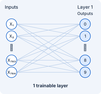
Our SLP (single-layer perceptron) network is fed an image, 28 by 28 pixels in size, a total of 784 pixels per image. Each pixel is a brightness value ranging from 0 (black) to 255 (white).
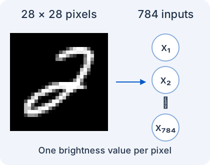
The SLP consists of ten neurons, one neuron for each digit, 0 to 9, to recognize. Each of these neurons receives the same input pixel values from all 784 pixels of the image. Each neuron outputs a score of the relative likelihood that the image presented is the digit the neuron is trained to recognize.
Each neuron has a weight for each input value, 784 per neuron, and a bias value. The weights and biases are adjusted in training to recognize digits written in a variety of different ways.

The letter options, available under the Advanced selection, work the same way with the number of neurons in the SLP being based upon how many letters or digits it is to recognize.
Result
The selection is based upon which neuron has the highest score. This is considered the digit read.
How it Learns
Our inputs. Each training image is 28 × 28 pixels for a total of 784 pixel values; each value is the brightness of that pixel, ranging from 0 (black) to 255 (white).
Prepare the inputs. We normalize (scale) the image brightness values so that bright images do not have greater overall value when we use those in our learning corrections.
Misreading an “8” should not have more learning value than misreading a “1” simply because an 8 uses more ink.
We calculate a scaling factor by adding together the squares of all pixel values, and then taking the square root. We divide each pixel value by this scaling factor. This is called L2 normalization or Euclidean normalization.
Writing the pixel values row by row as p₁ through p₇₈₄:
L = √(p₁² + p₂² + … + p₇₈₄²)
Xᵢ = pᵢ / L
These X values are the neuron inputs. They range from 0 to 1, with no negative values; the divisor depends on the whole image. If every pixel is 0, leave every input at 0. For example, if only two pixels are nonzero, with values 3 and 4, L is 5 and their inputs become 0.6 and 0.8.
Initialize the weights. Each of the ten neurons has its own 784 weights, one per input: 7,840 weights altogether. Set each weight to an independent uniform random value between −0.1 and +0.1, and each neuron’s bias, b, to 0. Learning can move weights and biases beyond those initial values.
Calculate the outputs. For each neuron, multiply each X input by its corresponding weight, add all 784 products, then add that neuron’s bias:
score = w₁X₁ + w₂X₂ + … + w₇₈₄X₇₈₄ + b
This is the diagram’s Σ + b. The score can be positive, zero, or negative, with no fixed output range or separate firing threshold. Read the digit with the highest score; ties go to the smaller digit.
- Present a labeled training image and calculate the reading using the current weights and biases.
- If the reading matches the label, change no weights or biases.
- If the reading is wrong, update only the correct digit’s neuron and the wrongly selected neuron. For each input position i, add Xᵢ to the correct neuron’s weight at that position and subtract Xᵢ from the wrong neuron’s weight at that position. Add 1 to the correct neuron’s bias; subtract 1 from the wrong neuron’s bias. The other eight neurons are unchanged.
Example: The label is 2, but the model reads 7, and X₁₇ is 0.6. If neuron 2’s weight for input 17 is 0.05, it becomes 0.05 + 0.6 = 0.65. If neuron 7’s weight for that input is 0.10, it becomes 0.10 − 0.6 = −0.50. Apply the same rule at every input position. Each pixel’s normalized value updates its corresponding weight in those two neurons; the sum of the inputs is never added to the weights.
Repeat for all 10,000 training images, making five passes with a new shuffle for each pass: 50,000 image presentations.
Average for display. For each weight and each bias, keep a separate running total of its value just before every image is processed. Divide each total by the number of images processed to obtain the averaged model used for testing and displayed readings. Continue training with the current, unaveraged values. The percentages are calculated afterward from the averaged scores and do not affect these updates.
Testing uses 1,000 separate images. Test results do not adjust the model or choose when training stops. Test images load when you select a dataset; training and calibration images load when you press Learn. Training and drawing stay in your browser.
MNIST images: Yann LeCun and Corinna Cortes, CC BY-SA 3.0. Original pixel values are preserved in the selected subsets. About the dataset · Subset details.
EMNIST: Gregory Cohen, Saeed Afshar, Jonathan Tapson, and André van Schaik, derived from NIST Special Database 19. About EMNIST · Subset details.
AI Winter
Early success in the field of AI led to a great deal of initial enthusiasm and research funding. This even spilled over to popular culture, where movies about the dangers of AI appeared, such as 2001: A Space Odyssey (1968) and Colossus: The Forbin Project (1970).
But by the late 1960s and early 1970s it was becoming clear that these early successes were hard to build upon and many techniques did not scale up. One important critique came in the 1969 book Perceptrons by Marvin Minsky and Seymour Papert, offering proofs of the limitations of single-layer and certain other perceptrons.
By the mid-1970s, enthusiasm and research funding had declined significantly. This period is called the AI Winter, or the first AI Winter. A second began in the late 1980s, as the promise of expert systems also failed to materialize.
Backpropagation: Learning Through Layers (1986)
1986 · Teaching the hidden layers
While single-layer perceptron neural networks were limited, multi-layer perceptrons offered greater promise. But how does one train them?
For single-layer perceptrons, the learning rule gives a clear method to adjust the weights as successes and failures against the training data are seen. But with multiple layers, where each neuron connects to every neuron in the next layer, how does one know what to adjust?
Single-Layer Perceptron
Multi-Layer Perceptron
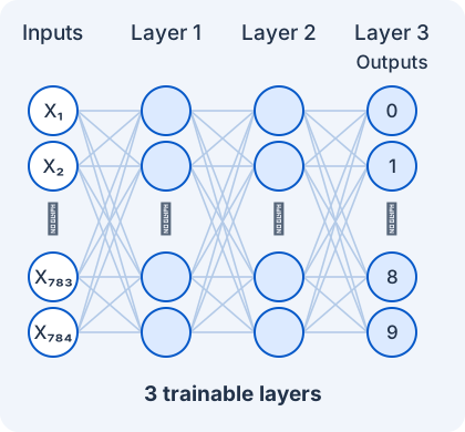
This is the credit-assignment problem: when an answer is wrong, which connections should change, and by how much?
Learning from the error
Backpropagation techniques popularized in 1986 provided for MLPs what the Learning Rule had provided for SLPs.
Backpropagation uses the chain rule from calculus to determine how each connection weight influences the output, working backward from the output through the layers to guide adjustments to the weights.
Miscellaneous
Explore
A grab bag of ideas and links to hold onto for now